Cousin Marriage Rates Have Varied Over Human History

The new paper, linked below, has made it possible to tease inbreeding rates out from incomplete ancient genomes, which has added an accurate measure of a key society level culture practice from prehistoric periods to the arsenal of anthropologists. Previously, ancient DNA could only show the relatedness of people in shared burials.

[C]ousin-marriage was far less common in the prehistoric and historic past than it is in some modern societies. In particular, it is far less common than it is today in the Islamic world and in India. That being said, the r.o.h values [runs-of-homozygosity (to measure inbreeding)] do decrease with agriculture from hunter-gatherer periods, indicating that large farming societies were more exogamous…before a recent shift in some areas to endogamy. . . .

The authors, for example, had transects from Pakistan, and in the past people in this region were not nearly as inbred. The dynamic that is important to remember is the confluence between population growth and the development of what Samo Burja calls “social technology”. In a modern world where societies are undergoing demographic transition and in the earlier stages of that process, so subject to massive growth, there will be lots of cousins to marry. In Malthusian societies, where families are just replacing themselves, there will not be as many cousins to marry. In other words, when there is a strong ideology of cousin-marriage, the limitation is going to be the number of cousins.

As many Islamic societies undergo demographic transition, I predict cousin-marriage will decrease as a phenomenon simply due to the reality that smaller families produce smaller kindreds from which one can select a mate.

But the second aspect here is social technology. In David Reich’s group’s work on India, it seems clear that strong endogamy as we see today did not really crystallize until ~1,500 years ago. . . . The practices of these societies are not from time immemorial but develop due to the exigencies of history and social evolution. Practices that we see as “conservative,” such as arranged-marriage, are actually innovations.

From here citing a table from Human Parental Relatedness through Time – Detecting Runs of Homozygosity in Ancient DNA.

* Previous analysis of cousin marriage, the frequency of which which varies greatly from culture to culture today, can be found at sister blog Wash Park Prophet, which noted that:

For the United States as a whole, the cousin marriage rate is about 0.2% (so there are about 250,000 people in these relationships), based mostly on old and not completely reliable data that are still unlikely to be wildly wrong, but "if you take a global perspective, consanguinity is not rare at all. Of the 70 countries studied, only 18 have consanguineous relationships as less than 1 percent of all marriages. In five countries, more than 50 percent of all marriages are between people who are second cousins or closer, and in Burkina Faso, it’s estimated that two of every three marriages are consanguineous."

A source for that post contained this map illustrating rates of consanguineous marriages globally:

The patterns of cousin marriage shown in the map above largely emerged around 500-1000 CE, in connection with the solidification of jati caste endogamy in South Asia and with the spread of Islam in the Middle East and North Africa, while the emergence of Christianity as the main source of marriage norms in the European dark ages, following the demise of the Roman Empire, reduced endogamy there.

A low rate of cousin marriage is one of the factors that some scholars believe drive some of the culturally distinctive aspects of WEIRD populations. See, e.g., Joseph Henrich, "The WEIRDest People in the World: How the West Became Psychologically Peculiar and Particularly Prosperous" (September 8, 2020).

In contrast, high rates of cousin marriage are associated with corrupt and weak governments, since obligations to one's extended family clan and even more extended family tribe can tend to override loyalty to a central state. See, e.g., Mahsa Akbai, et al., "Kinship, Fractionalization and Corruption" (October 3, 2016). Clan based societies seem to be the default "state of nature" in the absence of strong non-kinship related government, often overlapping with "cultures of honor" which are also associated with weak governmental power.

* Consanguinity measured by ROH is also related in endogamy rates. In modern India, as of 2011, the jati outmarriage rate is still just 5%. Jati are much more specific than varna or racial or macro-religious denomination type classifications. 

By comparison, native born Asian-American and Hispanic women in the U.S. have an outmarriage rate of almost 50%. Previous discussion of interracial marriage in the U.S. can be found at this post in sister blog Wash Park Prophet. It notes that:

About 15% of all new marriages in the United States in 2010 were between spouses of a different race or ethnicity from one another, more than double the share in 1980 (6.7%). Among all newlyweds in 2010, 9% of whites, 17% of blacks, 26% of Hispanics and 28% of Asians married out. Looking at all married couples in 2010, regardless of when they married, the share of intermarriages reached an all-time high of 8.4%. In 1980, that share was just 3.2%. 

Gender patterns in intermarriage vary widely. About 24% of all black male newlyweds in 2010 married outside their race, compared with just 9% of black female newlyweds. Among Asians, the gender pattern runs the other way. About 36% of Asian female newlyweds married outside their race in 2010, compared with just 17% of Asian male newlyweds. Intermarriage rates among white and Hispanic newlyweds do not vary by gender. . . . 

About one-in-five (22%) of all newlyweds in Western states married someone of a different race or ethnicity between 2008 and 2010, compared with 14% in the South, 13% in the Northeast and 11% in the Midwest. At the state level, more than four-in-ten (42%) newlyweds in Hawaii between 2008 and 2010 were intermarried; the other states with an intermarriage rate of 20% or more are all west of the Mississippi River. . . . 

The overall out marriage rate in the absence of any in marriage preference would be something on the order of 35-40% of newlyweds rather than the current 15%, although geographic considerations and social class considerations might trim the race neutral out marriage rate to closer to perhaps 30%. 

There is no race-gender combination in a person who is more likely to marry a person of another race than they would be if random chance determined pairings, and for almost all minority groups the difference between random pairings and actual out marriage rates is considerable. Even the people most prone to outmarry (for example, certain subcategories of U.S. born Asian and Hispanic women) have outmarriage rates on the order of 50%-60%, in a society where outmarriage rates would be closer to 80%+ in the absence of some endogamy effects. Once one controls for geography at the scale where people actively interact with potential spouses and for social class, quite a bit of this endogamy tendency is diluted, but any way you measure it, it is still there. As a general rule, people tend to marry people who are as similar to them as possible without being closely related. . .  

Native-born Hispanics were nearly three times as likely as their foreign-born counterparts to marry a non-Hispanic in 2010 [36.2% v. 14.2%]. 

The disparity among native- and foreign-born Asians is not as great, but still significant: Nearly four-in-ten native-born Asians (38%) and nearly a quarter (24%) of foreign-born Asians married a non-Asian in 2010.

Among Asian newlyweds, the intermarriage gap between native and the foreign born is much bigger for Asian men than for Asian women. In 2010, native-born Asian male newlyweds were about three times as likely as the foreign born to marry out (32% vs. 11%). Among newlywed Asian women, the gap between native and foreign born is much smaller (43% vs. 34%). The gender differences are not significant among Hispanic native- and foreign-born newlyweds. . . . 

[I]nterracial marriages that are most vulnerable to divorce involve white females and non-White males (with the exception of white females/ Hispanic white males) relative to white/white couples. Conversely, there is little or no difference in divorce rates among white men/non-white women couples, and white men/black women couples are actually substantially less likely than white/white couples to divorce by the 10th year of marriage.

Another point of comparison would be outmarriage rates for religious groups that make up a small share of the total U.S. population (Jews, Mormons and Muslims):

87% of Mormons and more than eight-in-ten Muslims (84%) in the United States are married to people with the same religion. 

Rates of intermarriage vary considerably among the major U.S. Jewish movements or denominations. Virtually all Orthodox respondents who are married have a Jewish spouse (98%), and most married Conservative Jews also have Jewish spouses (73%). Half of Reform Jews who are married have a Jewish spouse. Among married Jews who have no denominational affiliation, 31% have a Jewish spouse.

* Another way of measuring genetic segregation and divergence between populations is with an F(ST) statistic. Some populations in ancient times had genetic distances from each other that were as large as those between Europeans and East Asians today. The modern distinctions are summarized in this table:

From a 2003 paper (modern DNA sampling was possible long before good samples of ancient DNA were available).

For example, this was approximately the amount of genetic division between European hunter-gatherers and the first farmers of Europe, as illustrated by comparisons using, for example, ancient DNA:

The FST test indicated that European hunter-gatherer groups (hg_ce, hg_sca and hg_cant) did not show statistically significant differences between them, but they are significantly different from any population compared. . . . On the other hand, it was noted some differences within the European Neolithic groups, with the Neolithic group in Central Europe (neo_ce) showing the highest number of statistically significant differences in FST test, whereas the Neolithics from France and Catalonia (neo_fr and neo_cat) showed the lowest number of statistically significant differences.

Similarly, a 2010 ancient DNA study found that "early farmer and hunter-gatherers were from two well-differentiated populations (FST = 0.163; P<10-6)." 

Similarly, this was approximately the amount of genetic division between the hunter-gatherers the Levant and the hunter-gatherers of the Caucasus mountains and the highlands of what is now called Iran, a genetic division that carried over into the first farmer populations of these areas which was derived from local hunter-gatherers.

We computed squared allele frequency differentiation between all pairs of ancient West Eurasians, and found that the populations at the four corners of the quadrangle had differentiation of FST=0.08-0.15, comparable to the value of 0.09-0.13 seen between present-day West Eurasians and East Asians (Han). In contrast, by the Bronze Age, genetic differentiation between pairs of West Eurasian populations had reached its present-day low levels: today, FST is ≤0.025 for 95% of the pairs of West Eurasian populations and ≤0.046 for all pairs. These results point to a demographic process that established high differentiation across West Eurasia and then reduced this differentiation over time. 

Our data document continuity across the hunter-gatherer / farming transition, separately in the southern Levant and in the southern Caucasus-Iran highlands. The qualitative evidence for this is that PCA, ADMIXTURE, and outgroup f3 analysis cluster Levantine hunter-gatherers (Natufians) with Levantine farmers, and Iranian and Caucasus Hunter Gatherers with Iranian farmers. We confirm this in the Levant by showing that its early farmers share significantly more alleles with Natufians than with the early farmers of Iran: the statistic f4(Levant_N, Chimp; Natufian, Iran_N) is significantly positive (Z=13.6). The early farmers of the Caucasus-Iran highlands similarly share significantly more alleles with the hunter-gatherers of this region than with the early farmers from the Levant: the statistic f4(Iran_N, Chimp; Caucasus or Iran highland hunter-gatherers, Levant_N) is significantly positive (Z>6).

From Iosif Lazaridis, "Genomic insights into the origin of farming in the ancient Near East," 536(7617) Nature. 419–424. (August 25, 2016). doi: 10.1038/nature19310

A few years later, the genetic sources of Anatolian first farmers was established with ancient DNA:

Anatolia was home to some of the earliest farming communities. It has been long debated whether a migration of farming groups introduced agriculture to central Anatolia. Here, we report the first genome-wide data from a 15,000-year-old Anatolian hunter-gatherer and from seven Anatolian and Levantine early farmers. We find high genetic continuity (~80–90%) between the hunter-gatherers and early farmers of Anatolia and detect two distinct incoming ancestries: an early Iranian/Caucasus related one and a later one linked to the ancient Levant. Finally, we observe a genetic link between southern Europe and the Near East predating 15,000 years ago. Our results suggest a limited role of human migration in the emergence of agriculture in central Anatolia.

Feldman, M., et al. "Late Pleistocene human genome suggests a local origin for the first farmers of central Anatolia." 10 Nat Commun 1218 (March 192019). https://doi.org/10.1038/s41467-019-09209-7

In contrast, the first farmers of most of the rest of Europe (also here and here), North Africa and South Asia were predominantly migrants from elsewhere.

From this March 2011 paper.

There was also significant genetic distance between the first farmers of Europe and the Corded Ware and Bell Beaker people derived populations that partially replaced them in the early Bronze Age. For example, a 2015 paper explains that:

The Corded Ware are genetically closest to the Yamnaya, 2,600 km away, as inferred both from PCA and ADMIXTURE and FST (0.0116 0.002). If continuous gene flow from the east, rather than migration, had occurred, we would expect successive cultures in Europe to become increasingly differentiated from the Middle Neolithic, but instead, the Corded Ware are both the earliest and most strongly differentiated from the Middle Neolithic population.

 

As indicated in the table from that paper above, the genetic distance in terms of Fst between the most diverged Middle Neolithic population from the Corded Ware and Bell Beaker populations is 0.042 in the case of the Bell Beaker sample is 0.052 in the case of the Corded Ware population - only about half of the difference between the hunter-gatherers of the Levant from those of the Caucasus mountains, or between European hunter-gatherers and the first farmers of Europe, or between Europeans and the Han Chinese - but about twice as great as between any two West Eurasian populations in existence today.

This suggests these cultures were strongly endogamous with respect to these respective populations despite their sometimes reasonably close geographic proximity to each other.

The Relative Precision Of Comparable QED And QCD Calculations

QED and QCD calculations are generally done by truncating an infinite series of terms representing more and more byzantine paths by which a carrier boson can get from point A to point B.

The formula for determining uncertainty in the final result of a QED calculation (i.e. the Standard Model quantum theory of the electromagnetic force a.k.a. quantum electrodynamics) and the uncertainty in the final result of a QCD calculation (i.e. the Standard Model quantum the strong force that holds protons and neutrons together, and indirectly holds atomic nuclei together a.k.a. quantum chromodynamics) is, at an order of magnitude level, very similar.

The main differences are (1) the strength of the coupling constants of the respective theories, (2) the fact that in QED photons don't interact with photons while in QCD gluons interact with gluons, and (3) the fact that QED has only positive and negative electromagnetic charges, while QCD has red, antired, blue, antiblue, green and antigreen charges (which confusingly due to group theory produces eight rather than nine color-anticolor pair combinations for gluons).

Relative precision in a QED or QCD calculation equals one part per a^(2*L) which a is a constant that is about 12 for QED and about 2 for QCD, and L is the number of loops in the calculation. The factor should be roughly 5 for the weak force.

These factors primarily arise from the relative strengths of the respective coupling constants of the two theories, with a four loop calculation including terms with powers of eight of the coupling constant, although it isn't quite that simple, but the other factors primarily influence the number of calculations that have to be made per loop.

It other words, it takes more loops in QCD to get the same level of precision as one would in QED, and each new loop in QCD is harder to calculate than the corresponding one in QED.

In the case of QED:

* a one loop calculation is precise to about 1 part per 144.

* a two loop calculation is precise to about 1 part per 20,736.

* a three loop calculation is precise to about 1 part per 2,985,984 (a.k.a. about 3 parts per 10 million).

* a four loop calculation is precise to about 1 part per 429,981,696 (a.k.a. about 2 parts per billion).

* a five loop calculation is precise to about 1 part per 61,917, 364,224 (a.k.a. about 2 parts per 100 billion).

In the case of QCD:

* a one loop calculation is precise to about 1 part per 4.

* a two loop calculation is precise to about 1 part per 16.

* a three loop calculation is precise to about 1 part per 64.

* a four loop calculation is precise to about 1 part per 256 (a.k.a. about 4 parts per thousand).

* a five loop calculation is precise to about 1 part per 1024.

A seven loop calculations in QCD is less precise than a two loop calculation in QED. A one loop calculation in QED is almost as precise as a four loop calculation in QCD.

Higher loop calculations that can be ignored in QED can't be ignored in QCD, which is good because each additional loop is profoundly more cumbersome to calculate than the loop before it.

A deeper analysis can be found at Physics Stack Exchange. It also points out that the infinite series that are being approximated are not truly convergent, and that the errors start getting bigger rather than smaller after about five loops. 

But, this currently doesn't matter much. Nobody can do measurement approaching the one part per 61 billion precision of a five loop QED calculation, so we don't need that calculation to be more precise. And, nobody can actually do a QCD calculation of more than five loops, so the loss of precision in going beyond that point is merely hypothetical. 

It does illustrate, however, the limits of the current perturbative QCD techniques made using this method - which is about one part per thousand with the theoretically maximal accuracy of using this approach.

Syllables In English v. Japanese v. Hawaiian

Language log discusses syllables and related concepts in English, in Japanese, and in Hawaiian. My instincts were good, but not perfect.

It is also a good illustration of the fact that you really need to know the underlying language source of a word to convert it from a written word to a spoken one accurately, because Roman letters don't code the same sounds in every language in the same way.

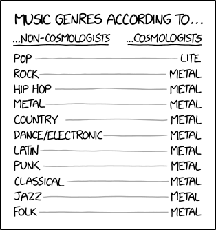
Yes, This Is An Inside Joke.

From here.

What is he on about?

[W]e . . . have to keep track of the stuff that isn’t hydrogen – helium and everything else in the periodic table, which astronomers often refer to collectively as “metals.” This makes for all sorts of partially-deserved jokes – oxygen isn’t a metal! but it is number 3 in cosmic abundance after hydrogen and helium. Like many anachronisms, the practice has good historical precedent. Early efforts to measure the abundances of the chemical elements in stars first gave results for iron. As other elements were probed, their abundances followed a pattern that scaled pretty well with the abundance of iron relative to hydrogen. So once again we have a proxy – this time, the iron abundance being a stand-in for that of everything else. Hence the persistence of the terminology – the metallicity of a star is a shorthand for the fraction of its mass that is not hydrogen and helium. 

And that fraction is small. We usually write the mass fractions of hydrogen, helium, and everything else (metals) as 

X + Y + Z = 1 

where X is the fraction of mass in hydrogen, Y that in helium, and Z is everything else. For the sun, Lodders gives X = 0.7389, Y = 0.2463, and Z = 0.0148. Do I believe all those significant digits? No. Is there a good reason for them to be there? Yes. So without delving into those details, let’s just note that the universe is about 3 parts hydrogen, one part helium, with a sprinkling of everything else. Everything else being all the elements in the periodic table that aren’t hydrogen or helium – all the carbon and nitrogen and oxygen and silicon and magnesium and noble gases and actual metals – these all add up to about 1.5% of the mass of the sun, which is typical of nearby stars. So you can see why they’re all just metals to many astronomers. 

For the mass of gas in galaxies, we need to correct what we measure in hydrogen for the presence of helium and metals. We measure the mass of atomic hydrogen using the 21 cm line, but that’s just the hydrogen. There is a corresponding amount of helium and metals that goes along with it. So we estimate the mass fraction in hydrogen, X, and use divide by that to get the total mass: M(gas) = M(HI)/X. We do the same for molecular gas, etc. 

There are measurements of the metallicities of entire galaxies, but – you guessed it – this isn’t observationally cheap, and isn’t always available. So we need another proxy. Luckily for us, it turns out that once again there is a pretty good correlation of metallicity with stellar mass: galaxies with lots of stars have made lots of supernovae that have processed lots of material into metals. Most of it is still hydrogen, so this is a very subtle effect: 1/X = 1.34 for the tiniest dwarf, going up to about 1.4 for a galaxy like the Milky Way. Still, we know this happens, so we can account for it, at least in a statistical way.

From Triton Station. 

Another Blow To Primordial Black Hole Dark Matter

Primordial black hole dark matter theories are dying deaths of a thousand cuts from observational evidence. This is one example of this process playing out. 

The funny normative phrasing of the final sentence of the abstract is probably just a function of "lost in translation" in the case of a paper written by a non-native speaker of the English language.

The frequent detection of binary mergers of ∼30M⊙ black holes (BHs) by the Laser Interferometer Gravitational-Wave Observatory (LIGO) rekindled researchers' interest in primordial BHs (PBHs) being dark matter (DM). In this work, we looked at PBHs distributed as DM with a monochromatic mass of 30M⊙ and examined the encounter-capture scenario of binary formation, where the densest central region of DM halo dominates. 

Thus, we paid special attention to the tidal effect by the supermassive black hole (SMBH) present. In doing so, we discovered a necessary tool called loss zone that complements the usage of loss cone. We found that the tidal effect is not prominent in affecting binary formation, which also turned out insufficient in explaining the totality of LIGO's event rate estimation, especially due to a microlensing event constraining the DM fraction in PBH at the mass of interest from near unity to an order smaller. Meanwhile, early-universe binary formation scenario proves so prevailing that the LIGO signal in turn constrains the PBH fraction below one percent. Thus, people should put more faith in alternative PBH windows and other DM candidates.

Yuan Gao, Xiaojia Zhang, Meng Su, "Has LIGO Detected Primordial Black Hole Dark Matter? -- Tidal Disruption in Binary Black Hole Formation" arXiv (June 29, 2020)

Neutrino Physics Hints Go Away

The data pointing to the neutrino mass ordering, its CP violating parameter, and tensions between two different ways of measuring one of the neutrino oscillation parameters has gotten weaker.

To recap, the big open questions in neutrino physics are: 

1. Is there a normal ordering or inverted ordering of neutrino masses? 

The downgraded 2.7 sigma preference implies that there is a 98% chance that the mass ordering is normal rather than inverted.

2. What is the lightest neutrino rest mass eigenstate? 

There is good reason to believe that it is significantly less than the difference between the lightest and second lightest neutrino rest mass eigenstate (which in a normal ordering is about 8.66 milli-electron volts, a.k.a. meV) and is greater than zero.

3. Is PMNS matrix parameter θ23 a little more than 45º or a little less (with the same magnitude of difference from 45º in either case)?  

There is roughly an 85% chance that it is more, and a roughly 15% chance that it is less, given the 1.6 sigma preference for the higher value. 

4. What is the CP violating phase of the PMNS matrix? 

The available observations suggest that the CP violation due to the CP violating phase of the PMNS matrix is more likely to happen than it is to not happen, and could be maximal, but the measurement uncertainty is too great to be very specific. There are myriad theoretical predictions of this phase which take on almost every conceivable value of the parameter.

5. Are there non-sphaleron processes like neutrinoless double beta decay involving neutrinos that do not conserve lepton number? 

The Standard Model answer to this question is "no", but the existing experimental tests aren't powerful enough to resolve the question because the expected number of neutrinoless double beta decay events is expected to be very small for neutrino masses of the magnitude that the combined available evidence especially from cosmology favors. In most of the beyond the Standard Model theories that are discussed in published scientific journal articles, the answer is "yes".

6. By what means do neutrinos acquire their rest mass? 

There is not a Standard Model answer to the question. The other fundamental particles of the Standard Model acquire their mass via interactions with the Higgs field, but due to the absence of a right handed neutrino and left handed anti-neutrino in the Standard Model, an extension of this mechanism to the neutrinos is not obvious or straightforward. Until neutrino oscillation and neutrino mass were confirmed, the Standard Model assumed taht neutrinos were massless. There is still some semantic dispute over whether neutrino mass and neutrino oscillation are actually truly part of the Standard Model of Particle Physics in the narrow sense of that term.

7. Do sterile neutrinos that oscillate with ordinary neutrinos exist? 

The Standard Model answer to the question is "no", and quite a bit of evidence from multiple sources (both cosmology and terrestrial experiment data) supports this answer. But there is some experimental evidence from neutrino oscillation data using neutrinos emitted by nuclear reactors (with the data from different experiments being somewhat inconsistent) that supports the existence of at least one sterile neutrino that oscillates with ordinary active neutrinos and such a neutrino is a dark matter particle candidate.

8. What is the ratio of neutrinos to antineutrinos in the Universe? 

We don't have a reliable measurement of any great precision. The electron neutrino asymmetry could be on the order of 3% and the muon and tau neutrino asymmetry could be on the order of 50%.

9. Is some other aspect of the Standard Model description of neutrinos incorrect? 

The Standard Model answer is obviously "no" and there is no strong evidence to suggest otherwise. The most plausible deviations from the Standard Model are discussed in the question above. Experimental searches for "non-standard interactions" (NSI) of neutrinos have not differed in a statistically significant manner from the null hypothesis.

10. Finally, it is always desirable to measure each of the seven experimentally measured neutrino property parameters of the Standard Model more precisely.

The measurement of the CP violating phase of the PMNS matrix is the least precisely measured experimentally determined constant in the entire Standard Model (or for that matter, in general relativity either, the other part of "Core Theory").

11. Bonus: Why do the seven experimentally measured neutrino property parameters take the values that they do? 

There is not a Standard Model answer to the question and it does not aspire to provide one.  The Standard Model does not aspire to explain why any of its experimentally measured fundamental constants take on the values that they do, except to demonstrate that a few of them (like the electromagnetic coupling constant, weak force coupling constant, W boson mass, Z boson mass, and Higgs vev) are functionally related to each other.

The preprint and its abstract are as follows:

Our herein described combined analysis of the latest neutrino oscillation data presented at the Neutrino2020 conference shows that previous hints for the neutrino mass ordering have significantly decreased, and normal ordering (NO) is favored only at the 1.6σ level. Combined with the χ2 map provided by Super-Kamiokande for their atmospheric neutrino data analysis the hint for NO is at 2.7σ. 

The CP conserving value δCP=180∘ is within 0.6σ of the global best fit point. Only if we restrict to inverted mass ordering, CP violation is favored at the ∼3σ level. 

We discuss the origin of these results - which are driven by the new data from the T2K and NOvA long-baseline experiments -, and the relevance of the LBL-reactor oscillation frequency complementarity. 

The previous 2.2σ tension in Δm^2(21) preferred by KamLAND and solar experiments is also reduced to the 1.1σ level after the inclusion of the latest Super-Kamiokande solar neutrino results. 

Finally we present updated allowed ranges for the oscillation parameters and for the leptonic Jarlskog determinant from the global analysis.

Ivan Esteban, M.C. Gonzalez-Garcia, Michele Maltoni, Thomas Schwetz, Albert Zhou "The fate of hints: updated global analysis of three-flavor neutrino oscillations" arXiv (July 27, 2020). This is largely in accord with another recent review of the same matters by different authors.

Other conclusions from the body text:

Despite slightly different tendencies in some parameter regions, T2K, NOvA and reactor experiments are statistically in very good agreement with each other. We have performed tests of various experiment and analysis combinations, which all show consistency at a CL below 2σ. 

We obtain a very mild preference for the second octant of θ23, with the best fit point located at sin^2(θ23) = 0.57 (slightly more non-maximal than the best fit of 0.56 in NuFIT 4.1), but with the local minimum in the first octant at sin^2(θ23) = 0.455 at a ∆χ 2 = 0.53 (2.2) without (with) SK-atm. Maximal mixing (sin^2(θ23) = 0.5) is disfavored with ∆χ 2 = 2.4 (3.9) without (with) SK-atm. 

The best fit for the complex phase is at δCP = 195◦ . Compared to previous results (e.g., NuFIT 4.1), the allowed range is pushed towards the CP conserving value of 180◦ , which is now allowed at 0.6σ with or without SK-atm. If we restrict to IO, the best fit of δCP remains close to maximal CP violation, with CP conservation being disfavored at around 3σ.

LambdaCDM Can't Explain Why The Milky Way's Satellite Galaxies Are In A Plane

The Standard Model of Cosmology also known as the lambdaCDM model is repeatedly in conflict with galaxy scale phenomena. The "Planes of Satellite Galaxies Problem" is one example of this reality. This result is expected and predicted, however, in many modified gravity theories.

Comparing satellite dwarf galaxies with ΛCDM simulations also results in numerous other small-scale problems (Missing Satellites, Core-Cusp, Too-Big-To-Fail) all of which are affected by baryonic physics.

We study the correlation of orbital poles of the 11 classical satellite galaxies of the Milky Way, comparing results from previous proper motions with the independent data by Gaia DR2. Previous results on the degree of correlation and its significance are confirmed by the new data. A majority of the satellites co-orbit along the Vast Polar Structure, the plane (or disk) of satellite galaxies defined by their positions. The orbital planes of eight satellites align to <20∘ with a common direction, seven even orbit in the same sense. Most also share similar specific angular momenta, though their wide distribution on the sky does not support a recent group infall or satellites-of-satellites origin. 

The orbital pole concentration has continuously increased as more precise proper motions were measured, as expected if the underlying distribution shows true correlation that is washed out by observational uncertainties. The orbital poles of the up to seven most correlated satellites are in fact almost as concentrated as expected for the best-possible orbital alignment achievable given the satellite positions. 

Combining the best-available proper motions substantially increases the tension with ΛCDM cosmological expectations: <0.1 per cent of simulated satellite systems in IllustrisTNG contain seven orbital poles as closely aligned as observed. 

Simulated systems that simultaneously reproduce the concentration of orbital poles and the flattening of the satellite distribution have a frequency of <0.1 per cent for any number of k > 3 combined orbital poles, indicating that these results are not affected by a look-elsewhere effect. 

This compounds the Planes of Satellite Galaxies Problem.

Marcel S. Pawlowski, Pavel Kroupa "The Milky Way's Disk of Classical Satellite Galaxies in Light of Gaia DR2" arXiv (November 12, 2019) (Accepted for publication in MNRAS).

Antimatter Does Not Have Negative Gravitational Mass

Kroupa comes up with a clever way to rule out a theory rooted in the notion that antimatter has negative gravitational mass without directly measuring it, using solar system based constraints.

The gravitational dipole theory of Hadjukovic (2010) is based on the hypothesis that antimatter has a negative gravitational mass and thus falls upwards on Earth. 

Astrophysically, the model is similar to but more fundamental than Modified Newtonian Dynamics (MOND), with the Newtonian gravity gN towards an isolated point mass boosted by the factor ν=1+(α/x)tanh(x√/α), where x≡gN/a0 and a0=1.2×10^−10 m/s2 is the MOND acceleration constant. We show that α must lie in the range 0.4−1 to acceptably fit galaxy rotation curves. 

In the Solar System, this interpolating function implies an extra Sunwards acceleration of αa0. This would cause Saturn to deviate from Newtonian expectations by 7000(α/0.4) km over 15 years, starting from known initial position and velocity on a near-circular orbit. 

We demonstrate that this prediction should not be significantly altered by the postulated dipole haloes of other planets due to the rather small region in which each planet's gravity dominates over that of the Sun. The orbit of Saturn should similarly be little affected by a possible ninth planet in the outer Solar System and by the Galactic gravity causing a non-spherical distribution of gravitational dipoles several kAU from the Sun. 

Radio tracking of the Cassini spacecraft orbiting Saturn yields a 5σ upper limit of 160 metres on deviations from its conventionally calculated trajectory. These measurements imply a much more stringent upper limit on α than the minimum required for consistency with rotation curve data. Therefore, no value of α can simultaneously match all available constraints, falsifying the gravitational dipole theory in its current form at extremely high significance.

Indranil Banik, Pavel Kroupa "Solar System limits on gravitational dipoles" arXiv (June 10, 2020) (Accepted for publication by the Monthly Notices of the Royal Astronomical Society.)

Supermassive Black Holes Form Early

It takes about 100 million years after the Big Bang (the Universe is now about 13.8 billion years old) for supermassive black holes to form.

The observation of quasars at very high redshift such as Poniuaena is a challenge for models of super-massive black hole (SMBH) formation. This work presents a study of SMBH formation via known physical processes in star-burst clusters formed at the onset of the formation of their hosting galaxy. 

While at the early stages hyper-massive star-burst clusters reach the luminosities of quasars, once their massive stars die, the ensuing gas accretion from the still forming host galaxy compresses its stellar black hole (BH) component to a compact state overcoming heating from the BH--BH binaries such that the cluster collapses, forming a massive SMBH-seed within about a hundred Myr. Within this scenario the SMBH--spheroid correlation emerges near-to-exactly. The highest-redshift quasars may thus be hyper-massive star-burst clusters or young ultra-compact dwarf galaxies (UCDs), being the precursors of the SMBHs that form therein within about 200 Myr of the first stars. 

For spheroid masses <10^9.6 Msun a SMBH cannot form and instead only the accumulated nuclear cluster remains. The number evolution of the quasar phases with redshift is calculated and the possible problem of missing quasars at very high redshift is raised. SMBH-bearing UCDs and the formation of spheroids are discussed critically in view of the high redshift observations. 

A possible tension is found between the high star-formation rates (SFRs) implied by downsizing and the observed SFRs, which may be alleviated within the IGIMF theory and if the downsizing times are somewhat longer.

Pavel Kroupa, Ladislav Subr, Tereza Jerabkova, Long Wang "Very high redshift quasars and the rapid emergence of super-massive black holes" arXiv (July 28, 2020) (MNRAS, in press).

Footnote: Demerits to Professor Kroupa (whose work overall is excellent) for the incredibly long run on sentence in the abstract (part  of which is highlighted above).

Larger Stonehenge Stones Came From 15 Miles Away

A long standing mystery related to Stonehenge has been solved and the answer is less fabulous than we might have hoped. 

The mineral origin of Stonehenge is an ancient mystery now solved, thanks to the solving of more contemporary one: who absconded with core samples from a crumbling standing stone, drilled out in 1959 so it could be reinforced with rebar? One of the three cores was recently returned by an 89-year-old worker from the diamond company that performed the work six decades ago, and tests show that it came from a quarry only 15 miles north of the monument. 

. . . Stonehenge's smaller bluestones were already proven to be from a quarry in Wales. Their 142-mile journey probably involved a leg by boat, a logistical feat that would have been much more challenging for the larger cuts.

From here. 

ATLAS Finds No Evidence Of Lepton Universality Violations In W-Boson Decays

In the Standard Model of Particle Physics, electrons, muons and tau leptons have identical properties except rest mass. But there is mixed experimental evidence from W boson mediated decays of B mesons (i.e. two quark composite particles containing bottom quarks) to suggest that different charge leptons decay differently (much like quarks of different generations do pursuant to the CKM matrix). 

This study is the first and only experimental data point from the Large Hadron Collider addressing the question from the perspective of the ratio of tau leptons to muons. It does so in a "cleaner" experimental design with less room for unexpected systemic errors or theoretical issues than the B meson decay experiments that have shown signs of lepton universality violations. 

The results support the Standard Model rule known as "lepton universality" with results within less than one standard deviation of the Standard Model expectation. There are multiple models for what could cause lepton universality violations in B meson decays, however, and it can't rule out all of them definitively.

The Standard Model of particle physics encapsulates our current best understanding of physics at the smallest scales. A fundamental axiom of this theory is the universality of the couplings of the different generations of leptons to the electroweak gauge bosons. 

The measurement of the ratio of the rate of decay of W bosons to τ-leptons and muons, R(τ/μ)=B(W→τντ)/B(W→μνμ), constitutes an important test of this axiom. A measurement of this quantity with a novel technique using di-leptonic tt¯ events is presented based on 139 fb^−1 of data recorded with the ATLAS detector in proton--proton collisions at s√=13 TeV. Muons originating from W bosons and those originating from an intermediate τ-lepton are distinguished using the lifetime of the τ-lepton, through the muon transverse impact parameter, and differences in the muon transverse momentum spectra. 

The value of R(τ/μ) is found to be 0.992±0.013[±0.007(stat)±0.011(syst)] and is in agreement with the hypothesis of universal lepton couplings as postulated in the Standard Model. This is the most precise measurement of this ratio, and the only such measurement from the Large Hadron Collider, to date.

ATLAS Collaboration "Test of the universality of τ and μ lepton couplings in W-boson decays from tt¯ events with the ATLAS detector" arXiv (July 28, 2020).

The body text of the paper provides the following background to this experiment:

It is a fundamental axiom and remarkable feature of the Standard Model (SM) that the couplings of the electroweak gauge bosons (W, Z) to charged leptons, g(l) (l = e, µ, τ), are independent of the mass of the leptons. This fundamental assumption is referred to as lepton-flavour universality and is tested in this paper by measuring the ratio of the fraction of on-shell W boson decays, branching ratios (B), to τ-leptons and muons, R(τ/µ) = B(W → τντ)/B(W → µνµ). The measurement exploits the large number of top and anti-top quark pair (tt¯) events produced in proton-proton (pp) collisions at the Large Hadron Collider (LHC). Given the large B(t → W q), close to 100%, this gives a very large sample of W boson pairs. These are used in a tag and probe technique to obtain a large sample of clean and unbiased W boson decays to muons and τ-leptons. The τ-leptons are identified through their decay to muons. The displacement of the τ decay vertex and the different muon transverse momentum (pT) spectra are used to distinguish between muons from the W → τντ → µνµντ ντ and W → µνµ processes, to extract R(τ/µ). This is achieved by utilising the precise reconstruction of muon tracks obtainable by the ATLAS experiment. 

Previously, R(τ/µ) has been measured by the four experiments at the Large Electron–Positron Collider (LEP), yielding a combined value of 1.070 ± 0.026. This deviates from the SM expectation of unity[1] by 2.7σ, motivating a precise measurement of this ratio at the LHC. Other experimental measurements of the ratio B(W → τν(τ))/B(W → lν(l)), where l is either an electron or a muon, have not yet reached the precision of the LEP results. 

The equivalent ratio for the two light generations, B(W → µνµ)/B(W → eνe), has been accurately measured by the LEP, LHCb and ATLAS experiments, and is found to be consistent with the SM prediction at the 1% level. Additionally, while most low-energy experiments show good agreement, to very high precision, with the hypothesis of universality of lepton couplings, recent results from LHCb, Belle and BaBar show some tension with the SM, further motivating this analysis. 

This measurement relies on precise knowledge of the branching ratio of τ-leptons decaying to muons to extrapolate to the full W → τντ branching ratio. The value of (17.39 ± 0.04)% measured by the LEP experiments is used in the analysis. The relative uncertainty of 0.23% is included in the measured value of R(τ/µ) and is a subdominant component of the overall uncertainty.

[1] The phase space effects due to the masses of the decay products on this ratio are very small (∼ 5 × 10−4 ) and hence can be neglected [2]. 

Previous coverage of the question of lepton universality violations at this blog:

* Lepton Flavor Violations In B Meson Decays Still Seen In Experimental Evidence (updated March 27, 2019)

* A Review Of Lepton Universality In B Meson Decays (September 18, 2018)

* B Quark Decays Still Anomalous (June 25, 2018)

* Maybe b quark decays aren't weird after all (January 18, 2018)

* Some B Meson Decay Anomalies Disappear In Run-2 Data (May 10, 2017)

Viking Era Smallpox DNA

Somebody decided that "the Viking Age" sounded like a better time descriptor to put in the title of their paper than that time period's other common name, "the Dark Ages." 

Reading between the lines, one of the big questions being asked is whether smallpox suddenly evolved to become more deadly and virulent sometime in the 1600s.

Scientists have discovered extinct strains of smallpox in the teeth of Viking skeletons -- proving for the first time that the killer disease plagued humanity for at least 1400 years.

Smallpox spread from person to person via infectious droplets, killed around a third of sufferers and left another third permanently scarred or blind. Around 300 million people died from it in the 20th century alone before it was officially eradicated in 1980 through a global vaccination effort -- the first human disease to be wiped out.

Now an international team of scientists have sequenced the genomes of newly discovered strains of the virus after it was extracted from the teeth of Viking skeletons from sites across northern Europe. . . .

Smallpox was eradicated throughout most of Europe and the United States by the beginning of the 20th century but remained endemic throughout Africa, Asia, and South America. The World Health Organisation launched an eradication programme in 1967 that included contact tracing and mass communication campaigns -- all public health techniques that countries have been using to control today's coronavirus pandemic. But it was the global roll out of a vaccine that ultimately enabled scientists to stop smallpox in its tracks.

Historians believe smallpox may have existed since 10,000 BC but until now there was no scientific proof that the virus was present before the 17th century. It is not known how it first infected humans but, like Covid-19, it is believed to have come from animals. . . . 

The team of researchers found smallpox -- caused by the variola virus -- in 11 Viking-era burial sites in Denmark, Norway, Russia, and the UK. They also found it in multiple human remains from Öland, an island off the east coast of Sweden with a long history of trade. The team were able to reconstruct near-complete variola virus genomes for four of the samples. . . .

"The early version of smallpox was genetically closer in the pox family tree to animal poxviruses such as camelpox and taterapox, from gerbils. It does not exactly resemble modern smallpox which show that virus evolved. We don't know how the disease manifested itself in the Viking Age -- it may have been different from those of the virulent modern strain which killed and disfigured hundreds of millions."

Dr Terry Jones, one of the senior authors leading the study, a computational biologist based at the Institute of Virology at Charité -- Universitätsmedizin Berlin and the Centre for Pathogen Evolution at the University of Cambridge, said: "There are many mysteries around poxviruses. To find smallpox so genetically different in Vikings is truly remarkable. No one expected that these smallpox strains existed. It has long been believed that smallpox was in Western and Southern Europe regularly by 600 AD, around the beginning of our samples.

"We have proved that smallpox was also widespread in Northern Europe. Returning crusaders or other later events have been thought to have first brought smallpox to Europe, but such theories cannot be correct. While written accounts of disease are often ambiguous, our findings push the date of the confirmed existence of smallpox back by a thousand years."

From Science Daily.

Viking smallpox diversity 

Humans have a notable capacity to withstand the ravages of infectious diseases. Smallpox killed millions of people but drove Jenner's invention of vaccination, which eventually led to the annihilation of this virus, declared in 1980. 

To investigate the history of smallpox, Mühlemann et al. obtained high-throughput shotgun sequencing data from 1867 human remains ranging from >31,000 to 150 years ago (see the Perspective by Alcamí). Thirteen positive samples emerged, 11 of which were northern European Viking Age people (6th to 7th century CE). Although the sequences were patchy and incomplete, four could be used to infer a phylogenetic tree. This showed distinct Viking Age lineages with multiple gene inactivations. The analysis pushes back the date of the earliest variola infection in humans by ∼1000 years and reveals the existence of a previously unknown virus clade.

Science, this issue p. eaaw8977; see also p. 376 

Structured Abstract 

INTRODUCTION 

Variola virus (VARV), the causative agent of smallpox, is estimated to have killed between 300 million and 500 million people in the 20​th century and was responsible for widespread mortality and suffering for at least several preceding centuries. Humans are the only known host of VARV, and smallpox was declared eradicated in 1980. The timeline of the emergence of smallpox in humans is unclear. Based on sequence data up to 360 years old, the most recent common ancestor of VARV has been dated to the 16th or 17th century. This contrasts with written records of possible smallpox infections dating back at least 3000 years and mummified remains suggestive of smallpox dating to 3570 years ago. 

RATIONALE 

Ancient virus sequences recovered from archaeological remains provide direct molecular evidence of past infections, give detail of genetic changes that have occurred during the evolution of the virus, and can reveal viable virus sequence diversity not currently present in modern viruses. In the case of VARV, ancient sequences may also reduce the gap between the written historical record of possible early smallpox infections and the dating of the oldest available VARV sequences. We therefore screened high-throughput shotgun sequencing data from skeletal and dental remains of 1867 humans living in Eurasia and the Americas between ~31,630 and ~150 years ago for the presence of sequences matching VARV. 

RESULTS 

VARV sequences were recovered from 13 northern European individuals, including 11 dated to ~600–1050 CE, overlapping the Viking Age, and we reconstructed near-complete VARV genomes for four of them. The samples predate the earliest confirmed smallpox cases by ~1000 years. Eleven of the recovered sequences fall into a now-extinct sister clade of the modern VARVs in circulation prior to the eradication of smallpox, while two sequences from the 19th century group with modern VARV. The inferred date of the most recent common ancestor of VARV is ~1700 years ago.

The number of functional genes is generally reduced in orthopoxviruses with narrow host ranges. A comparison of the gene content of the Viking Age sequences shows great contrast with that of modern VARV. 

Three genes that are active in all modern VARV sequences were inactive over 1000 years ago in some or all ancient VARV. Among 10 genes inactive in modern and Viking Age VARV, the mutations causing the inactivations are different and the genes are predicted to be active in the ancestor of both clades, suggesting parallel evolution. Fourteen genes inactivated in modern VARV are active in some or all of the ancient sequences, eight of which encode known virulence factors or immunomodulators. 

The active gene counts of the four higher-coverage Viking Age viral genomes provide snapshots from an ~350-year period, showing the reduction of gene content during the evolution of VARV. These genomes support suggestions that orthopoxvirus species derive from a common ancestor containing all genes present in orthopoxviruses today, with the reduction in active gene count conjectured to be the result of long-term adaptation within host species.

CONCLUSION 

The Viking Age sequences reported here push the definitive date of the earliest VARV infection in humans back by ~1000 years. These sequences, combined with early written records of VARV epidemics in southern and western Europe, suggest a pan-European presence of smallpox from the late 6th century. The ancient viruses are part of a previously unknown, now-extinct virus clade and were following a genotypic evolutionary path that differs from modern VARV. The reduction in gene content shows that multiple combinations of active genes have led to variola viruses capable of circulating widely within the human population.

Barbara Mühlemann, et al., "Diverse variola virus (smallpox) strains were widespread in northern Europe in the Viking Age." 369 (6502) Science eaaw8977 (July 24, 2020).

The companion commentary and its abstract are as follows:

Smallpox—caused by variola virus (VARV), a poxvirus—was one of the most virulent diseases known to humans, killing up to 30% of infected individuals and 300 million to 500 million people in the 20th century. The year 2020 commemorates the 40th anniversary of smallpox eradication, the first human disease eradicated after a global vaccination campaign led by the World Health Organization (WHO). The last samples of VARV are kept in two high-security laboratories pending destruction, and fears about reemergence or deliberate release of VARV have not subsided (1). Smallpox eradication is one of the most successful stories of public health, but the origin of the deadly virus remains an enigma. On page 391 of this issue, Mühlemann et al. (2) report the identification of VARV in archaeological remains from the Viking Age (600 to 1050 CE) that reveals new information about the origin of VARV and its evolution in human populations.

Antonio Alcamí, "Was smallpox a widespread mild disease?" 369 (6503) Science 376-377 (June 24, 2020).

Is the Hydra An Allegory For Summer?

"[T] the mythical theme of a hero (god) slaying 7 headed dragon keeps popping up again and again in different cultures in Eurasia...

For instance the Ugaritic monster Lotan (meaning "coiled"), also called "the mighty one with seven heads", was a serpent of the sea god Yam. Or Yam himself as he was also called "the serpent". This monster was defeated by the storm god Hadad-Baʿal in the Ugaritic Baal Cycle...

Hadad defeating Lotan, Yahweh defeating Leviathan, Marduk defeating Tiamat, Zeus slaying Typhon, Heracles slaying Hidra, Perun killing Veles, Thor fighting Jörmungandr...Different versions of the same myth which originated most likely in the Fertile Crescent among the Neolithic farmers[.]"

From the Old European culture blog.

The myth of a great warrior slaying a seven headed beast is an ancient and widespread one. Where did it come from? 

The author of the Old European culture blog makes the case that it is an allegory for the climate trends of the seasons, with the seven heads representing the seven months of the Fertile Crescent's summer.

About Massive Gravity

There is a lot of ongoing publication of academic papers on massive gravity theories. There have been sixty-four pre-prints on the topic at arXiv in the last 12 months alone. This research is driven by the desire to develop a theory of quantum gravity, the absence of which is one of the most obvious defects of "core theory" (i.e. the Standard Model plus General Relativity) that remains one of the most important unsolved problems in physics.

It is one part of a larger project in quantum gravity and general relativity research to better understand gravity by exploring modifications of canonical classical general relativity and its most naive quantum generalizations, to see what they imply and to better understand the mathematics of gravity and general relativity more generally,

By crude analogy, abstract algebra, parts of which are vital tools in physics, is basically a working out of what happens if you remove or add rules to rules like the commutative and associative properties of ordinary algebra and seeing what it looks like and whether you can gain insights or tools from that exercise.

We, of course, don't have the instrumental capacity to detect individual gravitons the way that we can detect individual photons, because the coupling constant of gravity at the scale of individual fundamental particles is so much weaker than the three Standard Model forces. So, we can't simply directly measure the mass of a graviton, and even if we could, we couldn't do so with perfect precision (this isn't just a practical difficulty, it is theoretically impossible to do so). Therefore, we can't rule out the possibility of a massive graviton with a mass of less than the uncertainty of our most precise measurement by direct measurement alone.

So, the only way to distinguish between the two possibilities is to work out theoretically the observable implications of each possibility, to learn how they differ, and with this knowledge to try to see if we can use indirect evidence to distinguish between the possibilities.

Indeed, one reason to explore it is that it provides an alternative to the massless spin-2 graviton approach to quantum gravity (the overwhelmingly conventional wisdom) which allows you to quantify how far experimental data requires the conventional wisdom to be true, rather than the alternatives.

It is one thing to say that experimental data is not inconsistent with the hypothesis of a massive graviton. It is another to say that experimental evidence constrains any massive graviton theory to have a graviton with a mass of not more than 6*10^-32 eV at the two sigma confidence level, pursuant to a study of weak gravitational lensing data done in 2004, and that thirteen other papers analyzing different astronomy observations in an effort to constrain this parameter experimentally have imposed no other boundaries that are more strict.

Quantifying the allowed parameter space of massive gravity theories allows us to quickly rule out BSM theories which aren't within the limits of those parameters. So, this is an active area of experimental as well as theoretical investigation, although there haven't been a lot of really big breakthroughs on the experimental side recently.

More generally, comparing the math involved in quantum gravity with a massive graviton to the math involved in massive gravity with a massless graviton, helps you understand what is going on in each case better.

As a practical matter, one of the main barriers to a theory of quantum gravity is that the naive mathematical description of a massless spin-2 graviton that couples in proportion to the mass-energy of what it interacts with is non-renormalizable (and is also a non-Abelian gauge theory, i.e. its math doesn't obey the commutative law mathematically, and is highly non-linear) and no one has figured out how to do the non-perturbative math (or use not yet discovered #mathtricks) that are necessary to get meaningful answers out of this formulation in a more general case as opposed to some very specific, highly idealized and symmetric cases. So, looking at the closely related cases of massive graviton theories may help you to gain insight into why you can't solve the massless graviton case.

To take one concrete example of that, the graviton matter coupling in massive gravity is arguably easier to formulate than in the massless graviton case. Similarly, it is arguably to describe the interaction of quantum electrodynamics with gravity in a massive graviton formulation, and some of the insights that result from that analysis may generalize to both massive and massless graviton cases.

Also, it would be hubris to claim to know for sure that the massless graviton case is really true, when we can't even realize it mathematically in any way that we can use practically. This isn't Platonic knowledge that we are born with. While the massless graviton case is more attractive for many reasons, we can't rule out the possibility that the massless graviton mass is not just hard, but impossible to solve and non-physical. If so, perhaps the seemingly unlikely massive graviton case is actually correct, so we may as well pursue both possibilities theoretically.

On the other hand, if we pursue massive graviton theory to the point where we can definitively rule out it as a possibility due to some theoretical inconsistency that exists for all of the available parameter space, then we could indirectly establish that quantum gravity must arise from a massless graviton, even though we can't directly measure that fact.

Another reason to explore it is that even in the conventional massless spin-2 graviton approach to quantum gravity, gravitons still emit and absorb gravitons, because gravitons couple to mass-energy rather than mass alone, and gravitons have energy even though they lack rest mass in the conventional quantum gravity analysis. Gravitational fields have self-interactions in General Relativity, but the way that this occurs in GR is not very transparent or illuminating when GR is formulated in terms of Einstein's equations, but is much more transparent and obvious when developing an understanding of these self-interactions in a massive gravity quantum gravity context. A massive graviton approach can be used as a way to understand these self-interactions by viewing massless gravity as a limiting case of the massive graviton theory that is mathematically less vexed in some respects because any time you try to do math with zeros everywhere, you will usually end up with infinities that are mathematically hard to work with sooner or later (because division by zero is undefined and approaches "infinity" in the limit).

The problem with using a massive gravity theory to explore the limiting case of the massless graviton, however, is that there are qualitative differences between the way that bosons with even tiny masses behave compared to the way that a truly massless boson behaves.

For example, in layman's terms, massless bosons basically don't experience time and always move at exactly the speed of light regardless of how much energy they carry. But a massive boson does experience time, must move at either less than the speed of light (or more than the speed of light if it is a tachyon), and as a consequence of special relativity, it takes increasingly more energy to increase its speed by the same amount, as it approaches the relativistic regime near the speed of light.

Lensing effects are also not continuous between the massive graviton case and the massless graviton case, so the lensing effects of massive gravitons in the limit as the mass of the graviton falls in the direction of zero from above is not equal to the lensing effects created by a massless graviton.

In a massless graviton theory, tachyonic gravitons (i.e. those traveling at more than the speed of light) can be ruled out almost automatically by assumption. In a massive graviton theory, this isn't a foregone conclusion, and if it is true, you have to work a lot harder to reach that conclusion.

In general, it is quite challenging to formula a massive gravity theory that has desirable properties such as being "ghost free", and the discovery in 2010 that it appeared to be possible to devise a ghost free massive gravity theory rebooted interest in the theory that had gone dormant not long after it was determined in 1972 that a large class of massive gravity theories produce mathematical "ghosts" that it is impossible to remove from this class of theories. While this wasn't a true "no go" theorem, and the conclusion had loopholes that were later successfully exploited, interest in massive gravity theories waned to a trickle for a generation as a result of this discovery.

There are even efforts to explore the possibility of dark matter phenomena as a function of quantum gravity with a massive graviton. Likewise:

The fact that general relativity is modified at large distances in massive gravity provides a possible explanation for the accelerated expansion of the Universe that does not require any dark energy. Massive gravity and its extensions, such as bimetric gravity,[12] can yield cosmological solutions which do in fact display late-time acceleration in agreement with observations.[13][14][15]

This is attractive, because while it is trivial to insert a cosmological constant into Einstein's equations in classical GR as an integration constant, it is highly non-trivial to produce dark energy in a graviton based quantum gravity theory in which all global phenomena must arise from the local properties of a graviton (it is easier, at least in principle, to reproduce dark energy in quantum gravity theories like loop quantum gravity, that are quantizing space-time rather than merely inserting a graviton into a smooth and continuous space-time).

Theorists are also looking at massive gravity theories to address other problems in cosmology and black hole and neutron star physics that have gone unsolved in the massless graviton/massless gravitational field paradigm (all illustrated by the list of pre-prints linked above).